The Regression to the Mean
Peter Bernstein’s Against the Gods captivating history of risk rekindled and made me look with new eyes the regression to the mean trading approach —where many good methods take their cue.
Let’s walk this through the simple throws of a six face die. The probability of landing any face after a throw is 1/6, and it’s average 3.5 (adding 1 through 6, and dividing by 6).
Now comes the good part.
The central limit theorem states that the sums of many sets of equally distributed numbers will form a normal distribution. Imagine you throw your die 30 times, and repeat this sampling 100 times. If you add up the numbers where the die lands on for each sample, you will have 100 numbers —the total for each sample. These 100 numbers will have a normal distribution even though the die throws numbers with equal frequency (1/6).
So, how can we use this information?
We know that the bell shaped normal distribution peaks at its mean, that’s why 3.5 times 30 would be the most likely occurrence of the sum total for the samples, followed by 3 and 4 times 30, followed by 2 and 5 times 30, and so on…
In other words, we expect to get more samples that hover around a 3.5 average. So, in any given sample, if the first series of numbers thrown turn out to be under 3.5, it’s reasonable to expect that the next numbers should be higher…
December 10 — A word of caution. Let’s not forget that you never want to catch falling knives, you should expect an indication of strength before entering a long side swing trade —you need to see a double bottom formation.
For securities, the first thing is to find an adequate?? average. Why?
Security price sample sums also follow a normal distribution, but, they have a bias. As Jesse Livermore would put it, “you need to know if the market is going up or down…” I would add that we also need to know if it’s going nowhere, or sideways. In essence, know the trend.
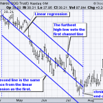
Hence, we draw a best fit straight line (linear regression) for the prices of a security —the average, with a 2 standard deviation channel around it, which tells us that a price has a rather small 2.5 percent probability of being out of the top or bottom channel boundaries.
The Raff Regression Channel is a good proxy for this kind of chart. Developed by Gilbert Raff, the Raff Regression Channel is a linear regression with evenly spaced trend-lines above and below. The width of the channel is based on the high or low that is the furthest from the linear regression.
In this example, the Raff Regression Channel extends from the April (closing) high to the July (closing) low. The late June high defines the width of the channel because it is the furthest high or low from the linear regression. This means the lower trend-line is set at the same distance from the linear regression as the upper trend-line.
Note that June’s high must’ve pushed to open the channel. A stop order trailing this extreme advance to sell at somewhere near these days lows would have pocketed a pretty penny! The failure of the test to break through the resistance of the top of a few days earlier —a double top failure— would have confirmed the short reversal position.
And finally, I almost forgot to mention a very important feature of the trade: we improve our chances by following the short trend. If anything goes south, the direction of the current will likely carry us to safe harbor…


![[Most Recent Quotes from www.kitco.com]](http://www.kitconet.com/charts/metals/base/spot-copper-30d.gif)
![[Most Recent Quotes from www.kitco.com]](http://www.kitconet.com/charts/metals/base/spot-copper-5y.gif)
![[Most Recent Quotes from www.kitco.com]](http://www.kitconet.com/charts/metals/base/lme-warehouse-copper-30d.gif)
![[Most Recent Quotes from www.kitco.com]](http://www.kitconet.com/charts/metals/base/lme-warehouse-copper-5y.gif)

[…] Peter Bernstein’s Against the Gods captivating history of risk rekindled and made me look with new eyes the regression to the mean trading approach —where many good methods take their cue. For more, visit con-tango, my trading blog… […]